Genre classification with Support Vector Machines
From now on, we will talk about the classification techniques we chose in order to achieve our goals.
First we tried to use Support Vector Machines, after using both extraction procedures.
First of all, the initial data set (which included 1000 pieces) has been split into two subsets of 750 (training) and 250 (test) pieces. In order to achieve this goal we used the train_test_split routine. Then we instantiated an SVC object, with all its parameters but probability set to their default values: we made this choice because we will run a Grid Search to choose the most promising ones. The probability parameter has been set to True because later we had to plot some ROC curves (which require some probability values). Some parameters associated to their default values are the following: C=1.0, kernel=’rbf’, degree=3, gamma=’auto’, coef0=0.0, shrinking=True.
Then, as you can see in the code snippet below, a Grid Search has been run in order to explore the following combinations of hyper-parameters (the order is not relevant):
- a Radial basis function kernel along with the cross product of C = [0.1, 0.3, 1, 3, 10, 30, 50], gamma values ranging in [0.01, 0.03, 0.1, 0.3, 1, 3], and an ignored degree list;
- a Polynomial kernel along with the cross product of C values ranging in [0.1, 0.3, 1, 3, 10, 30, 50], gamma = [0.01, 0.03, 0.1, 0.3, 1, 3], and degree = [1,2,3,4,5];
- a Sigmoid kernel along with the cross product of C = [0.1, 0.3, 1, 3, 10, 30, 50], gamma = [0.01, 0.03, 0.1, 0.3, 1, 3], and an ignored degree list.
Finally, model selection has been done thanks to a 5-fold cross validation along with f1 score as the selection metric.
Classifier instantiation and Grid Search
svc = SVC(probability=True)
params = [
  {'C': [0.1, 0.3, 1, 3, 10, 30, 50],
   'gamma': [0.01, 0.03, 0.1, 0.3, 1, 3], 'degree': [1,2,3,4,5],
   'kernel': ['rbf', 'poly', 'sigmoid']},
]

gsearch = GridSearchCV(svc, params, n_jobs=2,
                       verbose=1, scoring='f1_micro', cv=5)
gsearch.fit(data_train, target_train)
best_params = gsearch.best_estimator_.get_params()
for dict_item in params:
   for param_name in sorted(dict_item.keys()):
     print '\t%s: %r' % (param_name, best_params[param_name])
preds = gsearch.predict(data_test)
print classification_report(target_test, preds, target_names=mg_fft.GENRES)
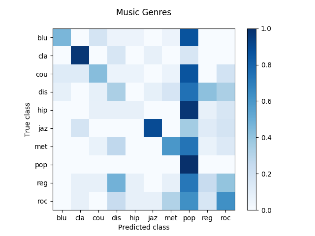
Performance with FFT
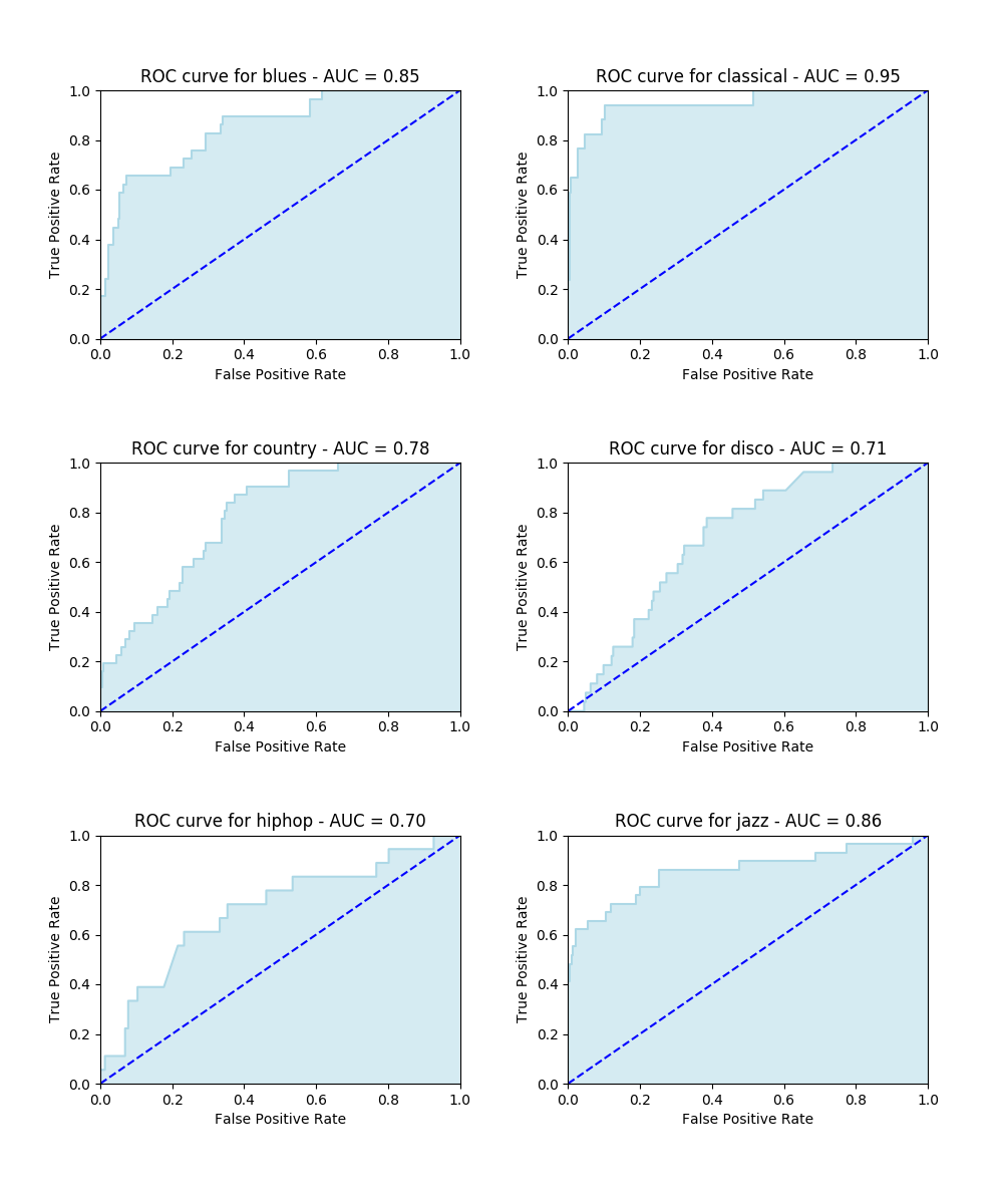
Here we present the results obtained after running an SVM classifier along with an FFT feature extraction. Firstly, a confusion matrix is shown, then some ROC curves and finally a classification report. Both graphs let us understand how the FFT can lead to disappointing results.
In the confusion matrix, the darker is the blue on the diagonal cells, the larger is the amount of right classifications. In the ROC curves, a larger Area Under Curve (AUC) indicates a better performance.
With respect to running time, 75 minutes were required to finish off this classification task. It ran so slowly because of the large amount of features (1000) required for each file.
| precision | recall | f1-score | support | |
|---|---|---|---|---|
| blues | 0.73 | 0.28 | 0.40 | 29 |
| classical | 0.63 | 0.71 | 0.67 | 17 |
| country | 0.50 | 0.23 | 0.31 | 31 |
| disco | 0.18 | 0.15 | 0.16 | 27 |
| hiphop | 0.20 | 0.06 | 0.09 | 18 |
| jazz | 0.83 | 0.52 | 0.64 | 29 |
| metal | 0.50 | 0.32 | 0.39 | 28 |
| pop | 0.16 | 1.00 | 0.27 | 16 |
| reggae | 0.21 | 0.11 | 0.15 | 27 |
| rock | 0.30 | 0.29 | 0.29 | 28 |
| Average / total | 0.44 | 0.33 | 0.34 | 250 |
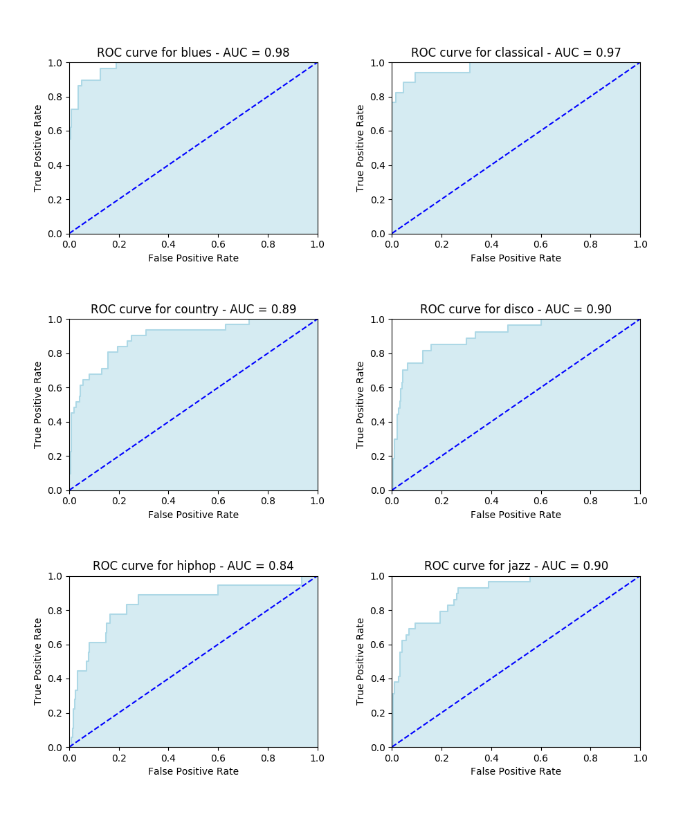
Performance with MFCC
As regards the alternative approach (MFCC), it definitely leads to much more promising outcomes, as you can see from the graphs below.
As regards running time, the classification task ran in about 5 minutes. This impressive decrease is due to the smaller amount of features (13) required in the MFCC extraction.

| precision | recall | f1-score | support | |
|---|---|---|---|---|
| blues | 0.73 | 0.76 | 0.75 | 29 |
| classical | 0.67 | 0.82 | 0.74 | 17 |
| country | 0.67 | 0.58 | 0.62 | 31 |
| disco | 0.58 | 0.56 | 0.57 | 27 |
| hiphop | 0.33 | 0.56 | 0.42 | 18 |
| jazz | 0.60 | 0.52 | 0.56 | 29 |
| metal | 0.75 | 0.75 | 0.75 | 28 |
| pop | 0.58 | 0.88 | 0.70 | 16 |
| reggae | 0.41 | 0.33 | 0.37 | 27 |
| rock | 0.35 | 0.21 | 0.27 | 28 |
| Average / total | 0.57 | 0.58 | 0.57 | 250 |